Extending the performance map
To complete the performance map, Costa relies on correction curves, following the methodology described by [Strugala]. Here’s a TLDR:
Select the performance map entries for each quantity to add.
Multiply the original performance map by a correction factor that depends on the entry value, for each selected entry.
Thus before filling the performance map, new entries and the corrections to use have to be specified, along with some other things. The following sections explain how to do so, and the last one shows how to finally fill the performance map.
Specify the operating mode
The corrections and the variables involved in the performance map depend on the operating mode (heating or cooling), which must therefore be specified before filling. (Not doing so will raise an exception.)
This can be done simply by assigning the string 'heating' or 'cooling'
to the attribute mode.
Warning
When using Permap attributes or methods,
don’t forget to use the pm prefix !
Set the performance map entries
The entries are stored in the entries attribute, in the form
of a dict with input quantities as keys and entries as values.
Valid keys for referencing input quantities are found in the
index names tables, and the selected entries must
be specified in the form of a list or a NumPy ndarray.
For example, to set frequency entries 0.1, 0.5 and 0.9 for a performance map
permap, you would do
>>> permap.pm.entries['freq'] = [0.1, 0.5, 0.9]
Manage the correction functions
Correction functions are the backbone of this performance map completion
methodology. Some default corrections are
available for you to use, but you can also
use your own.
Correction functions are stored in a dictionary like the
entries, in the corrections attribute.
However since corrections depends both on the input and output quantities of the
performance map, the dictionary is more nested; it has the following form:
{
   'AFR': {
      'power': <function>,
      'capacity': <function>,
      'COP': <function>,
   },
   'freq': {
      'power': <function>,
      'capacity': <function>,
      'COP': <function>,
   },
   ...
}
For example, to get the power correction as a function of frequency,
you could use permap.pm.corrections[‘freq’][‘power’] (see examples in
the Permap docstring). There is also a dedicated getter method,
get_correction, that would return the same correction
with permap.pm.get_correction(‘freq’, ‘power’).
It also allows to get all corrections associated with a specific input
by omitting the second argument.
Use default corrections
Everything related to the default corrections is contained in the
defaults module.
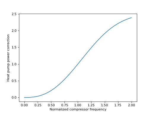
For getting a specific correction, there is the function
default_correction.
As with the Permap.get_correction method, it returns a callable
that can easily be visualized:
import numpy as np
import matplotlib.pyplot as plt
from costa.defaults import default_correction

corr = default_correction('heating', 'freq', 'power')
freq = np.linspace(0, 2, 100)
plt.plot(freq, corr(freq))
plt.xlabel("Normalized compressor frequency")
plt.ylabel("Heat pump power correction")
You can also get all the corrections associated with a certain
mode arranged in a dict structure as shown above,
using the function build_default_corrections.
Note
As of today, there are no regressions for the air flow rate (AFR) or the
indoor wet-bulb temperature (Twbr); all corrections associated with
these quantities are equal to 1.
Add custom corrections
Corrections can easily be edited or added through the
corrections attribute, but you may want to use the
set_correction method instead. Indeed, it performs some
security checks before updating the corrections dictionary, and it can also
return a new instance instead of modifying the performance table in-place
(see inplace argument.).
There is also the set_corrections method, which allows you
to specify all corrections associated with an input quantity. In addition,
it automatically adds correction functions that can be deduced from the others.
Indeed, since the output quantities are not independent
(\(\text{COP} = \dot{Q} / P\)) you can give only two corrections out of
the three and the last one will be automatically added.
For example, if you have a COP and a power correction named respectively
cop and power, you can do
new_corrections = {'COP': cop, 'power': power}
new_permap = permap.pm.set_corrections('freq', new_corrections)
and new_permap.pm.corrections[‘freq’] should have an entry 'capacity'.
Adjust the initial normalized values
By normalizing everything w.r.t. rated values, the correction functions must take the value 1 when the normalized input is 1 (i.e. for any correction function \(\varphi\), \(\varphi(1) = 1\)). But performance tables are not always provided at rated values. For example, it may happen that a spec sheet provide performance values at the maximum frequency \(f_\text{max}\), while the rated frequency \(f_\text{r}\) is only half of \(f_\text{max}\). In that case, the normalized frequency \(\nu = f / f_\text{r}\) would range from 0 to 2, and the initial performance data would be given at \(\nu = 2\). Since \(\varphi(2) \neq 1\), one cannot just multiply the performance map by \(\varphi(\nu)\) to extend it; we have to make sure that values are preserved at \(\nu = 2\). Thus, we must adjust the correction and instead multiply by \(\varphi(\nu) / \varphi(2)\).
More generally, if the performance data is provided at a certain condition
\(v^*\) different from the rated value \(v_\text{r}\), the correction
\(\varphi(v)\) must be adjusted by dividing it by
\(\varphi(v^*/v_\text{r})\). Therefore the ratio \(v^*/v_\text{r}\),
called the initial normalized value, must be explicitly specified for each
normalized quantity to extend the performance map correctly. This can be done
using the attribute initial_norm_values, where values are
once again stored in a dictionary whose keys are the normalized quantities
in question. So for example, if performance is provided at a frequency of
120 Hz but the rated frequency is 75 Hz, you would have to set
>>> permap.pm.initial_norm_values['freq'] = 120 / 75
Note
By default, i.e. if you don’t make any dict assignment, all those
values are set to 1. This means that, unless specified otherwise,
it is assumed that initial performance data is provided at rated values.
Fill the performance map
Once you have set the operating mode, the performance map entries, the
correction functions and the initial normalized values, you can
fill the performance map. To do so, simply
>>> permap_full = permap.pm.fill()
Note that you can combine the fill operation with the
normalize operation (see normalizing data),
by providing rated values to the fill method.
References
- Strugala
Strugala, G. (2020). Experimental testing and modelling of variable capacity air-to-air heat pumps (Master’s thesis, Polytechnique Montréal). Retrieved from https://publications.polymtl.ca/5285/